
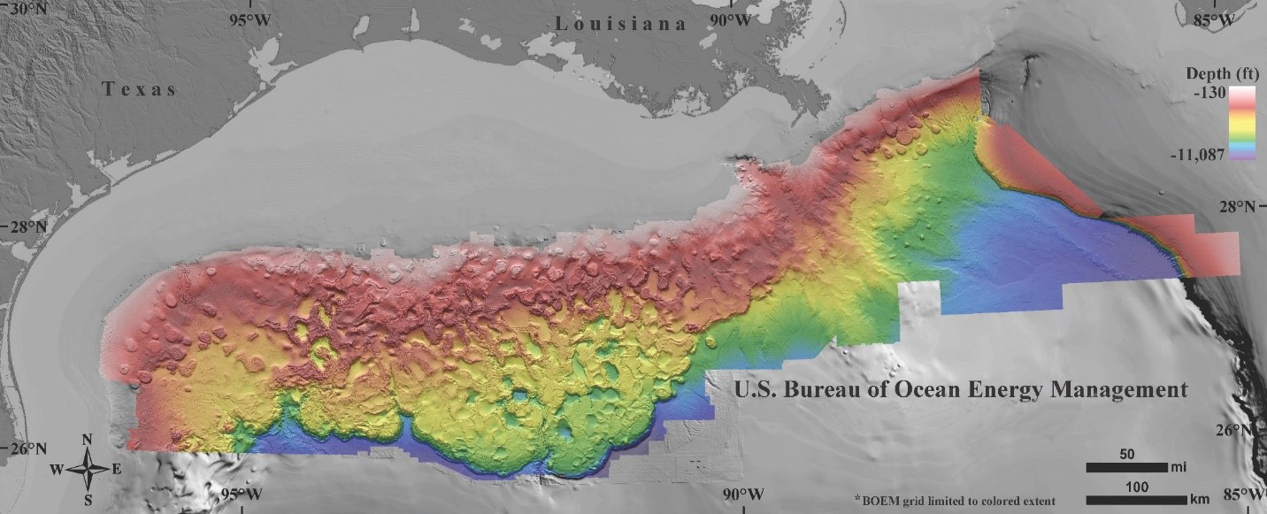
Figure 1. Northern Gulf of America deepwater bathymetry grid created from 3D seismic surveys. The grid defines water depth with 1.4 billion 40-by-40 ft cells and is available in feet and meters. BOEM grid coverage is the area defined by the color in this image. Shaded relief is vertically exaggerated by a factor of five.
- Introduction
- Grid Construction
- Notable Geologic Features
- Acknowledgements
- References
- Downloadable Files
The Bureau of Ocean Energy Management makes publicly available a new deepwater bathymetry grid of the northern Gulf of America, created by utilizing 3D seismic data which covers more than 90,000 square miles (Figure 1). The grid provides enhanced resolution compared to existing public bathymetry maps over the region, delivering 10 to 50 times increased horizontal resolution of the salt mini-basin province, abyssal plain, Mississippi Fan, and the Florida Shelf/Escarpment. To create the grid the seafloor was interpreted on over one-hundred 3D seismic time-migrated surveys, then mosaicked together and converted to depth in feet. The grid consists of 1.4 billion, 40-by-40 ft defined cells covering water depths –130 to –11,087 ft (–40 to –3,379 m). The average error is calculated to be 1.3 percent of water depth.
BOEM has the responsibility of issuing permits for the acquisition of geophysical data in U.S. Federal waters as designated under the Outer Continental Shelf (OCS) Lands Act. Regulations at 30 CFR 551 allow BOEM to obtain a digital version of any post-processed, post-migrated two-dimensional (2D) and three-dimensional (3D) seismic survey acquired within the OCS. BOEM now maintains a confidential library of approximately 1,700 time and depth 2D/3D seismic surveys for the gulf, with survey vintages dating back to the early 1980s. These data provide our geoscientists a world-class repository of subsurface digital data to interpret and utilize in achieving our regulatory missions.
Since 1998, BOEM has used the largest, highest quality 3D time surveys to interpret the seafloor. Time surveys were used because the primary objective was not bathymetry but to identify seafloor acoustic amplitude anomalies indicative of authigenic carbonate hardgrounds and natural hydrocarbon seepage; those areas which may be suitable habitat for communities of chemosynthetic, coral, and other benthic organisms [Roberts, 1996, Roberts et al., 1992 and 2000]. The acoustic amplitude response of the seafloor is better resolved in time-migrated surveys rather than depth-migrated, allowing for increased accuracy in the identification of potential benthic habitats and seeps. While this new bathymetry grid does not include acoustic amplitude data for the seafloor, BOEM does publish polygon shapefiles which outline areas of anomalously high and low seafloor acoustic reflectivity, which can be downloaded at www.boem.gov/Seismic-Water-Bottom-Anomalies-Map-Gallery.
The Bathymetry Grid
The grid defines water depth with 1.4 billion 40-by-40 ft cells and is available in feet and meters. Bathymetry ranges from –130 to –11,087 ft (–40 to –3,379 m) and includes vertically exaggerated slope-rendered hillshade files to illustrate seafloor features. The 3D seismic data used in its creation possess native horizontal resolution ranging from 41 to 123 ft, depending on the acquisition and processing parameters, and contains dominant frequencies of 10 to 50 Hz at the seafloor. Average horizontal resolution may be considered roughly 50 ft, with maximum bathymetry errors occurring on the shelf and uppermost slope in water generally shallower than 500 ft (150 m). Total average depth error is 1.3 percent of water depth. Due to the filesize of the grid, some downloadable products are split into Eastern and Western halves for data manageability and computer performance reasons. Contour datasets in varying intervals are also available.
Survey Selection and Mosaic Process
BOEM has been mapping the seafloor acoustic event, herein referred to as ‘horizon’, on time-migrated 3D surveys since 1998. Construction of the grid began by importing 200 individual seafloor horizons into geophysical 3D visualization software. Most of the Gulf has multiple, overlapping surveys of various vintages, so in an iterative method we compared horizons to each other in areas where surveys overlap. For all overlapped horizons we selected the interpretation with the best resolution and eliminated any overlapping horizons within its boundaries. The result is a mosaic of 117 of the highest quality seafloor horizons. Figure 2 illustrates this process.

Figure 2. A simplified illustration of the process which determined the final surveys to be included in the mosaic. This was an iterative process performed for over 200 surveys. 117 surveys were used in the final mosaic.
Each of the horizons in the mosaic still possessed its native horizontal cell size, most commonly 41 by 65.5 ft (12.5 by 20 m), with bins oriented along geographic north-south. However, many of the surveys acquired since the early 2000s are oriented along the direction of regional structural dip, roughly northwest-southeast, and possess larger average bin sizes in the 80 ft range. To merge all horizons into a single cohesive grid, all horizon cells had to have the same dimensions and compass orientation. Each horizon of the mosaic was resampled from its native resolution and cell orientation to a cell size of 40-by-40 ft with orientation along geographic north-south, per North American Datum 1927. This provided the cell homogeneity required for raster format while honoring the highest horizontal resolution of the input surveys. Also during this step we filled in minor gaps of missing seafloor data by using a convergent gridding algorithm and local dip of the closest cells.
Next we reconciled minor discrepancies in the two-way time (TWT) vertical Z dimension between adjacent seafloor horizons caused by annual migration of the GOA Loop Current. TWT adjustments were generally no greater than ± 10 to 20 milliseconds. Dependent upon the season in which a seismic survey was shot, the Gulf of America Loop Current and its eddies will induce faster or slower acoustic velocities within the water column, resulting in TWT differences in the order of tens of milliseconds for the same point on the seafloor. This is due to fluxes of the water column’s temperature and salinity as the Loop Current shifts throughout the year. A survey acquired in June will yield different seafloor TWTs when compared to a December survey over the same area. If left unchecked in the grid mosaicking process, the seams between surfaces of some adjacent surveys would be overly apparent, displayed as a perfectly vertical wall in the Z dimension. To partially correct for this in the final grid, we used a visually iterative process of comparing the edges of adjacent seafloor surfaces and then manually shifting one or both shallower or deeper. Some survey boundaries remain visible in the grid as thin linear features, as it was not possible to correct all vertical discrepancies given the physical size and temporal variations of this dataset.
Time-to-Depth Conversion
The East and West TWT grids were depth-converted using Advocate & Hood’s [1993] 7th-order polynomial time-to-depth equation for the northwest Gulf of America:
D = 0.1105 − 5066.9193T + 468.6693T2 − 554.7107T3 + 340.7019T4 − 116.9910T5 + 20.7280T6 − 1.4658T7
where
D = water depth (subsea feet)
T = one-way travel time (seconds).
The equation requires one-way travel time in seconds; however the grid up to this point was in two-way time in milliseconds. An initial conversion was performed by multiplying each grid by 0.0005 prior to applying the equation. After time-to-depth conversion there remained a few small geographic areas with gaps in which BOEM possesses no 3D time survey coverage. To fill those gaps in the grid, bathymetry was interpreted on 3D depth surveys and spliced in. As with the time survey cells, the depth survey cells had to be horizontally resampled to 40 ft and reoriented to geographic north-south.
Error Analysis
An error analysis (Figure 3 and Table 1) measures the depth-converted bathymetry against recorded water depths at 300 spatially distributed oil and gas wells located within the bounds of the grid. Error, expressed as percentage of water depth, decreases with deeper water and averages 1.3%. Highest average error of 5% occurs in water depths shallower than 500 ft due to the nature of conventional seismic acquisition in shallow water. Within the depth range of −2,000 to −11,000 ft, average error was calculated to be less than 0.5% of water depth.

Figure 3. Calculated error in the bathymetry grid after time-to-depth conversion. The bathymetry was measured against reported water depths at over 300 oil and gas wells. Error is expressed as percentage of water depth and decreases with depth.
Table 1. Average error of calculated water depth | ||||||||||||
|
Final Steps and GIS Products
The grid was exported from the geophysical 3D visualization software and imported to ArcMap. Using ArcMap we converted the grid to various user-friendly formats and generated additional GIS products, including bathymetric contours and hillshaded rasters. Hillshaded rasters showcase the dynamic bathymetric relief of the seafloor and were created using parameters of sun direction from due North at an angle of 45 degrees, with vertical exaggeration of 5. Pyramid files in ArcMap have been generated to allow users to quickly visualize the data at varying scales. For ArcMap users, the grid, contours, and all accompanying files were exported as a Map Package (.mpk) to preserve the visual characteristics of the grid so that the user will not have to import using default visual settings which may or may not be appropriate for this data. The map package is compatible with ArcMap 10.0 and newer. Contour shapefiles of varying intervals, in both feet and meters, are also available.
The detailed resolution of the BOEM bathymetry grid allows for enhanced visualization of interesting seafloor features and geomorphological processes. Figures 4 through 8 illustrate a very small sampling of those features. The shaded relief in all figures is vertically exaggerated by a factor of 5 to highlight geology.

Figure 4. Lloyd Ridge is a relict, meandering channel-levee complex stretching 174 mi (280 km) on the eastern abyssal plain. An additional 150 mi (240 km) is fully buried beneath younger Pleistocene turbidite deposits and Holocene slope facies. BOEM research has established updip linkage with the ancestral Pearl River [Frazier, 1974; Mobley, 2005]. Similar-scale channel-levee complexes have been observed in the Amazon Fan [Lopez, 2001]. The Florida Escarpment is visible to the northeast and younger Mississippi Fan to the southwest.

Figure 5. Current-derived furrows carved deep into the seafloor in the region around Green Knoll. First discovered in 1999 by Texas A&M deep-tow data and 3D seismic supplied by WesternGeco LLC, the furrows are expressed for over 200 km along the Sigsbee but are most pronounced on the plain, carving 1–10 m deep and 5–50 m wide [Bryant et al., 2000]. Currents within the furrows have been measured at rates up to 2 knots [Bryant et al., 2004].

Figure 6. Subaqueous dunes and pockmarks on the upper continental slope in the northwestern Gulf. Longitudinal mega-dunes are roughly 0.5–1 km crest-to-crest, 1–10 km long, 3–10 m tall. Pockmarks occur atop Nueces Dome (top center) and Gulf-wide pockmarks occur within a general water depth range of 300–600 m. Pockmarks in this region have been attributed to explosive dissociation of natural methane-hydrate following basinward migration of the hydrate stability zone during the Wisconsin Glacial Maximum sea-level lowstand [Hovland and Judd, 1988; Roberts and Carney, 1997]. BOEM has identified more than 4,000 pockmarks in the northern Gulf of America basin.

Figure 7. Features formed by the dynamic processes shaping the Gulf, specifically salt movement and natural hydrocarbon seepage. This site is located in the southern end of the Terrebonne Basin within the Walker Ridge protraction. Thrust faulting and folding is due to southeast verging lateral movement of allochthonous salt. Movement of salt is what gives the Gulf of America seafloor its rugose nature, also creating faults and fracture networks which provide pathways for oil and gas seeps. These particular expulsion mounds were formed as a result of basin compaction and compression, resulting in upward gas migration [McConnell and Kendall, 2002].

Figure 8. Alaminos and Perdido Canyons in new detail. The canyons funnel sediments to create an intermingling basin-floor fan system hundreds of meters thick. Core sampling determined that drainage from the Rio Grande River provides coarse, sandy sediments to the Perdido system [Damuth et al., 2006], whereas cores and well logs in Alaminos Canyon reveal primarily fine-grained deepwater clastics and hemipelagics [Bouma et al., 1968; Meyer et al., 2005].

Figure 9. A seafloor landscape common to the Gulf; a mound created from the interplay of basin subsidence and vertical migration of salt. As salt moves shallower relative to the subsiding basin around it, sediments are often uplifted and form seafloor mounds. Here, the movement created a network of extensional faults dividing the mound into three wedges. Faults also frequently provide pathways for fluid and/or gas migration, as indicated here by the circular depression on the southeast face of the mound, and expulsion feature with crater on the northwest side.
BOEM thanks the seismic data owners and geophysical acquisition companies which collected and processed the 3D surveys used to create this dataset. They are CGG Services (U.S.) Inc., Exxon Mobil Corporation, PGS, Seitel Inc., Spectrum USA, TGS, and WesternGeco LLC. This data will be a superb geospatial resource within the scientific, academic, and energy industry communities.
- Advocate, D., and K. Hood, (1993), An empirical time-depth model for calculating water depth, northwest Gulf of Mexico, Geo-Marine Letters, v. 13, p. 207–211.
- Bouma, A.H, W.R. Bryant, and J.W. Antoine, (1968), Origin and configuration of Alaminos Canyon, northwestern Gulf of Mexico, GCAGS Transactions, v. 18, p. 290–296.
- Bryant, W., T. Dellapenna, A. Silva, W. Dunlap, and D. Bean, (2000), Mega-furrows on the continental rise south of the Sigsbee Escarpment, Northwest Gulf of Mexico: AAPG Annual Meeting, New Orleans.
- Bryant, W., N. Niall, S. DiMarco, D. Bean, D. Berti, (2004), Deep-sea furrows: physical characteristics, mechanisms of formation and associated environmental processes, Texas A&M University, Department of Oceanography and Offshore Technology Research Center, RPSEA Final Report 0018-04.
- Damuth, J.E., C.H. Nelson, and H.C. Olson, 2006, Gulf of Mexico Intraslope Basins Project, GIB Phase 2 Project Atlas
- Frazier, D.E., (1974), Depositional episodes: their relationship to the Quaternary stratigraphic framework in the northwestern portion of the Gulf basin, Bureau of Economic Geology, University of Texas at Austin, Geological Circular 74–1.
- Hovland M., and A.G. Judd, (1988), Seabed pockmarks and seepages, impact on geology, biology and the marine environment, Graham and Trotman, London.
- Lopez, M., (2001), Architecture and depositional pattern of the Quaternary deep-sea fan of the Amazon, Marine and Petroleum Geology, v. 18, p. 479–486.
- McConnell, D.R., and B.A. Kendall, (2002), Images of the base of gas hydrate stability, northwest Walker Ridge, Gulf of Mexico, Offshore Technology Conference Transactions, Paper 14103, p. 1–10.
- Meyer, D., L. Zarra, D. Rains, B. Meltz, and T. Hall, (2005), Emergence of the Lower Tertiary Wilcox trend in the deepwater Gulf of Mexico, World Oil magazine, May 2005, p. 72–77.
- Mobley, C., (2005), Late Quaternary Louisiana shelf-margin deltaic deposition, north-central Gulf of Mexico, University of New Orleans Theses and Dissertations, Paper 237.
- Roberts, H.H., (1996), Surface amplitude data: 3D-Seismic for interpretation of seafloor geology (Louisiana slope): Gulf Coast Association of Geological Societies Transactions, v. 46, p. 353–362.
- Roberts, H.H., D.J. Cook, and M.K. Sheedlo, (1992), Hydrocarbon seeps of the Louisiana continental slope: Seismic amplitude signature and seafloor response: Gulf Coast Association of Geological Societies Transactions v. 42, p. 349–362.
- Roberts, H.H., J. Coleman, J. Hunt Jr., and W.W. Shedd, (2000), Surface amplitude mapping of 3D-seismic for improved interpretations of seafloor geology and biology from remotely sensed data, Gulf Coast Association of Geological Societies Transactions, v. 50, p. 495–503.
- Roberts, H.H., and R.S. Carney, (1997), Evidence of episodic fluid, gas, and venting on the northern Gulf of Mexico continental slope, Economic Geology, v. 92, no. 7–8, p. 863–879.
To View the Map in Your Internet Browser
- View the BOEM Seafloor Grid without having to download the data. You will be directed to the Marine Cadastre National Viewer, hosted by BOEM and NOAA's Office for Coastal Management.
For ArcGIS Users Only
- BOEM Gulf of Mexico Seafloor.mpk (Size: 4,225 MB) – This ESRI ArcMap map package contains all the bathymetry layers in one downloadable file. Users who download it do not need to download any additional files below. It is compatible with ArcMap version 10.0 and newer. Once on your machine, due to the size it may take up to 30 minutes or more to unpack and launch.
For Other Users and ArcGIS Users
- BOEM_Bathymetry_East_ft_tiff.zip (Size: 449 MB) – Eastern half of the bathymetry grid. Depth in feet.
- BOEM_Bathymetry_East_meters_tiff.zip (Size: 497 MB) – Eastern half of the bathymetry grid. Depth in meters.
- BOEM_Hillshade_East_tiff.zip (Size: 573 MB) – Hillshaded bathymetry of the Eastern grid. Vertically exaggerated by 5x.
- BOEM_Bathymetry_West_ft_tiff.zip (Size: 869 MB) – Western half of the bathymetry grid. Depth in feet.
- BOEM_Bathymetry_West_meters_tiff.zip (Size: 501 MB) – Western half of the bathymetry grid. Depth in meters.
- BOEM_Hillshade_West_tiff.zip (Size: 572 MB) – Hillshaded bathymetry of the Western grid. Vertically exaggerated by 5x.
- Gulf_Bathymetric_Contours.lpk.zip (Size: 363 MB) – ESRI ArcMap layer package containing bathymetric contours of varying intervals.
- Gulf_Bathymetric_Contours.zip (Size: 527 MB) – Zipped shapefiles for bathymetric contours of varying intervals.